Pivot Tables

To build pivot tables, it is sufficient to specify pivot table tags in the data range. After that, this range becomes the data source for the pivot table. The <<pivot>> tag is the first tag ClosedXML.Report pays attention to when analyzing cells in a data region. This tag can have multiple arguments. Here is the syntax:

<<pivot Name=PivotTableName [Dst=Destination] [RowGrand] [ColumnGrand] [NoPreserveFormatting] [CaptionNoFormatting] [MergeLabels] [ShowButtons] [TreeLayout] [AutofitColumns] [NoSort]>>

• Name=PivotTableName is the name of the pivot table allowed in Excel.
• Dst=Destination - the cell in which you want to place the left upper corner of the pivot table. If the Destination is not specified, then the pivot table is automatically placed on a new sheet of the book.
• RowGrand - allows you to include in the pivot table the totals by rows.
• ColumnGrand - includes totals for the pivot table.
• NoPreserveFormatting - allows you to build a pivot table without preserving the formatting of the source range, which reduces the time to build the report.
• CaptionNoFormatting - Formats the pivot table header in accordance with the source table.
• MergeLabels - allows you to merge cells.
• ShowButtons - shows a button to collapse and expand lines.
• TreeLayout - sets the mode of the pivot table as a tree.
• AutofitColumns - enables automatic selection of the width of the pivot table columns.
• NoSort - disables automatic sorting of the pivot table.

Here are some examples of the correct setting of the Pivot option:

• <<pivot Name=Pivot1 Dst=Totals!A1>> – a pivot table will be created with the name Pivot1; table will be placed on the Totals sheet starting at cell A1;
• <<pivot Name=Pivot25>> – a pivot table will be created with the name Pivot25;
• <<pivot Name=Pivot25 Dst=Totals!A1 RowGrand>> – the Pivot25 pivot table includes the totals for data lines;
• <<pivot Name=Pivot25 ColumnGrand>> – the pivot table will include the totals for the columns.

Fields in all ranges of the pivot table are added in the order in which they appear in the template (from left to right). Therefore, when designing a data range on which a pivot table will be built, you need to adhere to one simple rules: line up the columns in the order in which you would like to see them in the pivot table

Important!

The names of the fields for the pivot table are taken from the line above the data range - the heading of the source table. Be careful when creating this header, as there are some restrictions on the naming of fields in the pivot tables. With the help of pivot tables, it’s easy to create the most complicated cross-tables in reports.

Template example

Template file

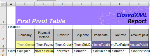
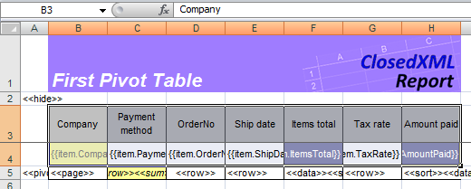
In the lower left cell of the data range there is a tag <<pivot Name="OrdersPivot" dst="Pivot!B8" rowgrand mergelabels AutofitColumns>>. This option will indicate ClosedXML.Report that a pivot table with the name “OrdersPivot” will be built across the region, which will be placed on the “Pivot” sheet starting at cell B8. And the parameter rowgrand will allow to include the totals for the columns of the resulting pivot table. In the service cell of the columns “Payment method”, “OrderNo”, “Ship date” and “Tax rate” the tag is <<row>>. The <<row>> tag defines the fields of the pivot table row area. In order to get the totals grouped by the method of payment of bills, the tag <<sum>> has been added to the tag <<row>> in the field “Payment method”. For the “Amount paid” and “Items total” fields, the <<data>> tag is specified (fields of the pivot table data range). In the options of the “Company” field, a <<page>> tag has been added (the page area field). When designing a template, in addition to the allocation of tags between the columns, do not forget to specify different formats for the cells of the range (including for cells with dates and numbers). Moreover, we formatted the service cells with column options, meaning that it is with this format that we will get subtotals in the pivot table. And for the “Payment method” field, we selected a cell with tags in color.

Static Pivot Tables

You can place one or several pivot tables right in the report template, taking advantage of the convenience of the Excel Pivot Table wizard and virtually all the possibilities in their design and structuring. Let’s give an example. As a starting point, we use the first example template with a summary table with the original Orders range on the Sheet1 sheet. Right in the template, we placed a static pivot table built over this range. The following figures show the steps for building this table. First, you need to select the source range for the pivot table. It is not identical to the Orders range, since it includes only the data line and the title above it. Notice how the source range is highlighted in the figure:

Next, we put the pivot table on a separate PivotSheet and distributed its fields in the rows, columns, and data ranges. We formatted pivot table fields, as well as their headings. Finally, we called the pivot table as PivotTable1, and as an option to the source range, we specified <<pivot>>. After the data is transferred, all summary tables referencing this data range will be updated. That is, for one range you can build several pivot tables.